Fleet Routing App - free Google Maps route planner for multiple stops
How to use the Google Maps free route planner to evaluate routes created in GMPRO.

In earlier blog posts in this tutorial series, I've demonstrated how to use GMPRO to solve the travelling salesman problem and the vehicle routing problem. In this one, I'll introduce a new tool: the GMPRO Fleet Routing App. This app serves as a free route planner, allowing Google Maps partners (aka resellers) and sales teams to evaluate routes created using the Google Maps Platform Route Optimization API (note: you will need a Google Maps Partner to grant you access to the app, direct customers cannot use the Fleet Routing App as is, but can host their own version with their own Google Maps API key by forking the Fleet Routing App GitHub repository).
Part 1: GMPRO: Google Maps Platform route optimization API
Part 2: GMPRO TSP solver: Google Maps with more than 25 waypoints
Part 3: Google Maps route optimization: multi vehicle
Part 4: Fleet routing app - free Google Maps route planner for multiple stops (this article)
Part 5: GMPRO docs: Fixed vehicle costs
Part 6: GMPRO docs: Territory optimization and route planning
Part 7: GMPRO docs: Solving the VRP with route clustering and soft constraints
Part 8: GMPRO docs: Driver load balancing with soft constraints
Part 9: GMPRO docs: Driver breaks
Part 10: GMPRO docs: Complete deliveries before pickups in cargo bike logistics
Part 11: GMPRO docs: Force stop sequences using precedence rules
Part 12: GMPRO docs: Cut cost / raise care with smart NEMT routing
Part 13: GMPRO docs: Routing for Demand Responsive Transport
Part 14: GMPRO docs: Squash durations and parking
What is the Fleet Routing App?
The Fleet Routing App is a web-based route planner used by Google's sales team and partner network to demonstrate GMPRO's capabilities to potential customers. In a typical technical sales conversation, the goal is to convince the customer that GMPRO can optimize their routes better than they can (though this isn't always true) and that the routes produced are practical and reflect real-world driving conditions (largely true, as GMPRO considers both real time and predicted traffic). To do this, it's essential to show the customer the optimized routes, which is where the Fleet Routing App comes into play.
The app has two modes. It can function as a viewer, where you use the GMPRO API to generate a route and then upload the request and response files to view it. It can also act as a route planner, allowing you to upload a list of drivers and shipments, and the app will optimize the routes for you. In this blog post, I'll guide you through using both modes.
Why use a free route planner with GMPRO?
Well, aside from it being free (the API key used in the Fleet Routing App belongs to Google, so presumably someone in Google's finance department gets a bill and promptly tosses it in the trash), the main advantage of using the Fleet Routing App is legibility. Here's what the JSON output of GMPRO looks like:
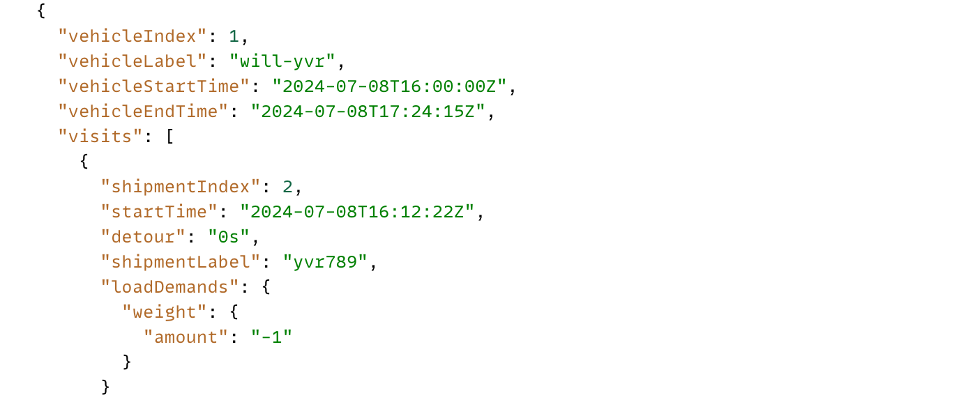
At a glance, I can tell that vehicle will-yvr starts his route at 16:00 hrs UTC on 2024--07-08 and makes his first delivery (loadDemands is negative), "yvr789", at 16:12 hrs UTC. That's about it, really.
But, if you use the Fleet Routing App, here's what you'll get instead:
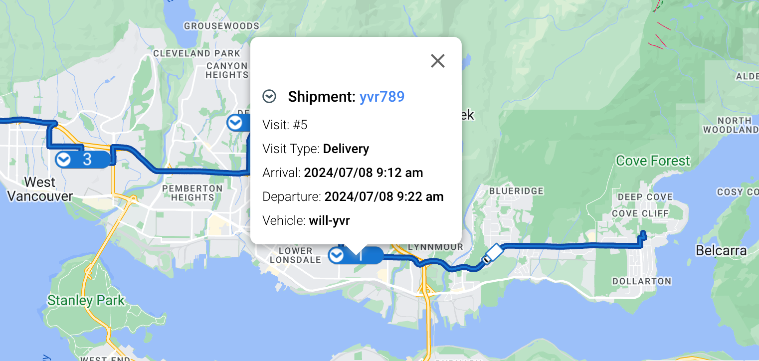
The app displays the routes generated by GMPRO on a map, allowing you to see not only where a delivery is scheduled but also when it will occur, adjusted for the delivery location's timezone. For example, if the delivery address is in Vancouver, Canada, which operates on Pacific Standard Time (PST), converting the arrival time of 16:12 UTC to PST results in 09:12 AM. This information, along with other useful details such as the visit type (pickup or delivery), vehicleLabel, shipmentLabel, and more, is prominently shown on the free route planner's user interface.
Using the Fleet Routing App as a route viewer
The first step to using the Fleet Routing App is to make a call to the /optimizeTours endpoint of the GMPRO route optimization API (refer to my tutorial on making your first GMPRO API request if you need help setting up your Google Cloud Project and CLI).
Making a GMPRO API call
Retrieve your API key and run the code snippet below to make a simple 6 visit / 2 vehicle optimization request.
curl -X POST 'https://routeoptimization.googleapis.com/v1/projects/{project_name}:optimizeTours' \
-H "Content-Type: application/json" \
-H "Authorization: Bearer $(gcloud auth application-default print-access-token)" \
--data-binary @- << EOM
{
    "model": {
        "shipments": [
            {
                "deliveries": [
                    {
                        "arrivalLocation": {
                            "latitude": 49.2545595,
                            "longitude": -123.1096174
                        },
                        "duration": "600s",
                        "timeWindows": [
                            {
                                "startTime": "2024-07-08T16:00:00Z",
                                "endTime": "2024-07-08T18:00:00Z"

                            }
                        ]
                    }
                ],
                "loadDemands": {
                    "weight": {
                        "amount": "1"
                    }
                },
                "label": "yvr123"
            },
            {
                "deliveries": [
                    {
                        "arrivalLocation": {
                            "latitude": 49.1654802,
                            "longitude": -123.1187887
                        },
                        "duration": "600s",
                        "timeWindows": [
                            {
                                "startTime": "2024-07-08T16:00:00Z",
                                "endTime": "2024-07-08T18:00:00Z"
                            }
                        ]
                    }
                ],
                "loadDemands": {
                    "weight": {
                        "amount": "1"
                    }
                },
                "label": "yvr456"
            },
            {
                "deliveries": [
                    {
                        "arrivalLocation": {
                            "latitude": 49.313724,
                            "longitude": -123.0514561
                        },
                        "duration": "600s",
                        "timeWindows": [
                            {
                                "startTime": "2024-07-08T16:00:00Z",
                                "endTime": "2024-07-08T18:00:00Z"
                            }
                        ]
                    }
                ],
                "loadDemands": {
                    "weight": {
                        "amount": "1"
                    }
                },
                "label": "yvr789"
            },
            {
                "deliveries": [
                    {
                        "arrivalLocation": {
                            "latitude": 49.343481,
                            "longitude": -123.0863414
                        },
                        "duration": "600s",
                        "timeWindows": [
                            {
                                "startTime": "2024-07-08T16:00:00Z",
                                "endTime": "2024-07-08T18:00:00Z"
                            }
                        ]
                    }
                ],
                "loadDemands": {
                    "weight": {
                        "amount": "1"
                    }
                },
                "label": "yvr987"
            },
            {
                "deliveries": [
                    {
                        "arrivalLocation": {
                            "latitude": 49.3352081,
                            "longitude": -123.1453979
                        },
                        "duration": "600s",
                        "timeWindows": [
                            {
                                "startTime": "2024-07-08T16:00:00Z",
                                "endTime": "2024-07-08T18:00:00Z"
                            }
                        ]
                    }
                ],
                "loadDemands": {
                    "weight": {
                        "amount": "1"
                    }
                },
                "label": "yvr654"
            },
            {
                "deliveries": [
                    {
                        "arrivalLocation": {
                            "latitude": 49.3513846,
                            "longitude": -123.2631103
                        },
                        "duration": "600s",
                        "timeWindows": [
                            {
                                "startTime": "2024-07-08T16:00:00Z",
                                "endTime": "2024-07-08T18:00:00Z"
                            }
                        ]
                    }
                ],
                "loadDemands": {
                    "weight": {
                        "amount": "1"
                    }
                },
                "label": "yvr321"
            }
        ],
        "vehicles": [
            {
                "startLocation": {
                    "latitude": 49.2808457,
                    "longitude": -123.0827831
                },
                "loadLimits": {
                    "weight": {
                        "maxLoad": 5
                    }
                },
                "startTimeWindows": [
                    {
                        "startTime": "2024-07-08T16:00:00Z"
                    }
                ],
                "endTimeWindows": [
                    {
                        "endTime": "2024-07-08T18:00:00Z"
                    }
                ],
                "label": "mark-yvr",
                "costPerKilometer": 1
            },
            {
                "startLocation": {
                    "latitude": 49.3191441,
                    "longitude": -122.9522224
                },
                "loadLimits": {
                    "weight": {
                        "maxLoad": 5
                    }
                },
                "startTimeWindows": [
                    {
                        "startTime": "2024-07-08T16:00:00Z"
                    }
                ],
                "endTimeWindows": [
                    {
                        "endTime": "2024-07-08T18:00:00Z"
                    }
                ],
                "label": "will-yvr",
                "costPerKilometer": 1
            }
        ],
        "globalStartTime": "2024-07-08T07:00:00Z",
        "globalEndTime": "2024-07-09T06:59:00Z"
    },
    "populatePolylines": true
}
EOM
Saving a GMPRO scenario
While waiting for the request to return a solution, copy and paste the JSON code between the "<<EOM" and "EOM" tokens into a text editor and save it as scenario.json.
Saving a GMPRO solution
Next, copy and paste the response returned by GMPRO into a new text file and save that as solution.json. This is what the returned route solution looks like:
{
  "routes": [
    {
      "vehicleLabel": "mark-yvr",
      "vehicleStartTime": "2024-07-08T16:00:00Z",
      "vehicleEndTime": "2024-07-08T16:55:26Z",
      "visits": [
        {
          "startTime": "2024-07-08T16:14:55Z",
          "detour": "0s",
          "shipmentLabel": "yvr123",
          "loadDemands": {
            "weight": {
              "amount": "-1"
            }
          }
        },
        {
          "shipmentIndex": 1,
          "startTime": "2024-07-08T16:45:26Z",
          "detour": "1096s",
          "shipmentLabel": "yvr456",
          "loadDemands": {
            "weight": {
              "amount": "-1"
            }
          }
        }
      ],
      "transitions": [
        {
          "travelDuration": "895s",
          "travelDistanceMeters": 4995,
          "waitDuration": "0s",
          "totalDuration": "895s",
          "startTime": "2024-07-08T16:00:00Z",
          "vehicleLoads": {
            "weight": {
              "amount": "2"
            }
          }
        },
        {
          "travelDuration": "1231s",
          "travelDistanceMeters": 11934,
          "waitDuration": "0s",
          "totalDuration": "1231s",
          "startTime": "2024-07-08T16:24:55Z",
          "vehicleLoads": {
            "weight": {
              "amount": "1"
            }
          }
        },
        {
          "travelDuration": "0s",
          "waitDuration": "0s",
          "totalDuration": "0s",
          "startTime": "2024-07-08T16:55:26Z",
          "vehicleLoads": {
            "weight": {}
          }
        }
      ],
      "routePolyline": {
        "points": "_dxkHnrfnV?`@HAN??f@Ar@@^@TDPFRBP@F?@@P?^?^?X?BAp@eBC@sFBeB@}@@mB?C@oB?O?g@?O?k@@}@?Y?S?m@@O?]A[?SAICWCa@Gc@B_@EWQ}@CMAKAME[AS?IAQAc@?g@?kA?_@RALOn@@H?|ABvA@|@?ZBvA@vAB|A@|A?vA?vAD|A@rA@xDBd@?t@@tA?jB?lA@tEBjB@R@fA@f@BRFNBV@h@Bh@B|@@^@vA@vA?r@ERALCPI`@?j@?xD@`@@r@@f@@Z?^@R?T?Z?J@N?V?n@@v@BpABr@?\\?H?PHn@BfA@zADBArA@RBtA@B?`@@R?\\?B@DAF?hAAX?B?p@AL?NAhACpA@?|@?z@?r@@l@A|BDV?^CfJA`K?~A?JAh@?v@?fB?jAAhI?x@ClC?^AdC?h@?^?v@?LAd@?X?~C?F?F?F?H?J?P?b@AV?D?F?F?D?nAAvF?v@CnI?~A?d@Ax@AVCPCr@Ar@_@|BIz@OdACXADGTER@x@AtC?h@?l@?`C?j@?`A?b@L?jDF\\AP?R?H?N@d@?B?V@T?NKxABr@@D?L?rCDb@@ApA?fA?LCfFAzDAvCAl@CxCEtE?V?RGvFGrFdBFxADD?|ABF@bBBh@@l@@|A@~ABhBBxABtA@vABzAB`@?b@@b@@fBBhBBdAF^B?d@?pAApA?bBCvB?bA?x@CzAAlA?`@AnD?h@AlA?R?XCpBAhC?ZATAlB?@AjB?HAl@?f@AhB?NClE?N?L?FAF?RA~B?d@?N?v@AnBEbE?@EnGC`CEpDAtA?F?t@C|A?`@N@PA^@V@~@BhA@fA@P?@?NEP?`ABR?l@@N?`B@zAARHDBF?|@@v@@lB@`@@lBB|@@PIfA@jCDzDDRAt@@h@?`A?pBBz@@f@?fA@L@T?hBHr@B`ABF?L@H?dA@@?jBB`HDXJJB|@@bA?N?fA@T@H?fDDn@?X?PA@AJEjA?fB@T@zFFN?~ADdA@vDDl@@tABDDBBD@\\@lA@h@@d@@R@P@\\?j@A\\?L?l@@rABF?VK~@B`CDN?ZDjB@rBB|FFd@?nA?r@B`@@f@?vA?b@@D?T@T?n@BZ@RBVB^DB?^FTDVFPDZHZHZHTH@@XJXJXLZLPJVJXLB@RF@@RFDBVH`@J\\JXFf@Jb@FZDZD^DVBT@F?Z@@?\\@R@lEDtABdEDfDDvABvA@hIHb@?tBDP@T?d@@V?d@J\\@P?zAGl@E`@AB?B?XC@?D?^CtASPETE^MLENERG\\Sf@UTKNKTMd@]^Y@CZWPOZYRQf@e@bA_ApAkAv@q@l@k@x@u@TSrBmBDCtAqAd@_@\\[pAmAlAiAdDyCPMj@i@v@s@`CyBrAkAdB_BPONOBCPQdB{Af@e@dAaAj@e@HIJK~CqCJKr@o@BCz@w@NONMJIJI~@{@|@y@ROp@k@p@o@h@m@`@g@BCLSNUV_@j@aADGNWhAgBZe@d@w@h@{@l@cAPYDGt@qAj@}@FST?NGLEJAHANAX?T@H@N@tAB^@fA?bA@nC@JEFAF?|ECjA?zAAhB@lC?|C?X?lG?J@xA?jA@PAxA?T@x@?~@@Z@jB?R?Z?l@?bBAx@?rB?pAA`@@|RCN?|C?ZAx@Al@?P@ZDn@@n@?h@AJ?N?~B?`H@pB?X?D?zB?RA?rA?R?nB?rBAzB?\\?T@dA?x@?`C?lBAh@?f@d@B"
      },
      "metrics": {
        "performedShipmentCount": 2,
        "travelDuration": "2126s",
        "waitDuration": "0s",
        "delayDuration": "0s",
        "breakDuration": "0s",
        "visitDuration": "1200s",
        "totalDuration": "3326s",
        "travelDistanceMeters": 16929,
        "maxLoads": {
          "weight": {
            "amount": "2"
          }
        }
      },
      "routeCosts": {
        "model.vehicles.cost_per_kilometer": 16.929
      },
      "routeTotalCost": 16.929
    },
    {
      "vehicleIndex": 1,
      "vehicleLabel": "will-yvr",
      "vehicleStartTime": "2024-07-08T16:00:00Z",
      "vehicleEndTime": "2024-07-08T17:24:51Z",
      "visits": [
        {
          "shipmentIndex": 2,
          "startTime": "2024-07-08T16:12:20Z",
          "detour": "0s",
          "shipmentLabel": "yvr789",
          "loadDemands": {
            "weight": {
              "amount": "-1"
            }
          }
        },
        {
          "shipmentIndex": 3,
          "startTime": "2024-07-08T16:31:49Z",
          "detour": "934s",
          "shipmentLabel": "yvr987",
          "loadDemands": {
            "weight": {
              "amount": "-1"
            }
          }
        },
        {
          "shipmentIndex": 4,
          "startTime": "2024-07-08T16:51:45Z",
          "detour": "1943s",
          "shipmentLabel": "yvr654",
          "loadDemands": {
            "weight": {
              "amount": "-1"
            }
          }
        },
        {
          "shipmentIndex": 5,
          "startTime": "2024-07-08T17:14:51Z",
          "detour": "2913s",
          "shipmentLabel": "yvr321",
          "loadDemands": {
            "weight": {
              "amount": "-1"
            }
          }
        }
      ],
      "transitions": [
        {
          "travelDuration": "740s",
          "travelDistanceMeters": 7934,
          "waitDuration": "0s",
          "totalDuration": "740s",
          "startTime": "2024-07-08T16:00:00Z",
          "vehicleLoads": {
            "weight": {
              "amount": "4"
            }
          }
        },
        {
          "travelDuration": "569s",
          "travelDistanceMeters": 7109,
          "waitDuration": "0s",
          "totalDuration": "569s",
          "startTime": "2024-07-08T16:22:20Z",
          "vehicleLoads": {
            "weight": {
              "amount": "3"
            }
          }
        },
        {
          "travelDuration": "596s",
          "travelDistanceMeters": 6332,
          "waitDuration": "0s",
          "totalDuration": "596s",
          "startTime": "2024-07-08T16:41:49Z",
          "vehicleLoads": {
            "weight": {
              "amount": "2"
            }
          }
        },
        {
          "travelDuration": "786s",
          "travelDistanceMeters": 12159,
          "waitDuration": "0s",
          "totalDuration": "786s",
          "startTime": "2024-07-08T17:01:45Z",
          "vehicleLoads": {
            "weight": {
              "amount": "1"
            }
          }
        },
        {
          "travelDuration": "0s",
          "waitDuration": "0s",
          "totalDuration": "0s",
          "startTime": "2024-07-08T17:24:51Z",
          "vehicleLoads": {
            "weight": {}
          }
        }
      ],
      "routePolyline": {
        "points": "eq_lHldmmVBADCB@^BAB@D@DBBB@BABCHGH?D?BC\\[JM`@c@R@H@TBAFAHAL?|@?v@A`AAt@dAFdB?fBCzAC?\\At@?v@?rAAlB@p@AdF?lB?b@CpC?lB?lBAv@?dD?zC?T?hC?PAdD?HAbBArC?hA?t@?v@A`KAvB?f@Av@?fA?~@Gb@?^?N?pB@x@?XBjB@Z?h@@t@@lA@vA@v@BxBL|HH|H?LBlB@lBD~ED~E@n@@jAAnD?lB?r@?z@AdC?t@Av@?v@?lBAt@?nBCjBAnB?t@?vAAdBAtBC|EAdDAbDAtCChB?nA?|BAjBAzE?\\AdDAdB?p@AhBAtB?BAt@?v@?hB?B?j@?D?P?T@V@VDp@Ff@D^Ff@F\\BJF\\H\\FRDR`@zA`AnCL\\?@L\\`@jAt@xBL^JXNb@n@bBHTLTZl@bArBZj@pA~BdB|CVb@p@tAh@`A`@r@r@lANZr@bBTp@Np@TlAHdABl@@n@CbACh@ALGd@EZGh@G\\Mv@Kp@Kj@AFCVE`@Ej@?BEn@AZ?N?T?R?Z?NBj@@^@T@B@TH`ALlABVFv@JdA@HFt@Hz@Dd@@HFr@Dd@B\\@^@\\?\\?BAXA\\CXCPMj@?DI\\GPCFGN]t@CFCDs@rAi@fAm@jAO\\M\\KTIVENENKd@W~AE^CXEh@Eh@?BEhAAh@?f@AjAAd@?N?T?l@?l@?`@BjA@RFtADv@BhAD`@B\\DTNv@Lj@DNFVFVLd@Nn@FZFT?BDTFf@?p@?ZALAJCTEPITELGLEFEFGHEFABABABAD?De@TMFMFWNKLGLKPEJGPM\\IRQn@Md@CNITA@ETEJAHANAZA^Ih@El@?X?B?hA?D?X@|@A^?b@@lBC`F?X?JCbKAzAAPEr@?BAr@?@?J?j@?h@?bA?d@Ab@ArBAvA?v@?t@?~@?p@?lECbA?lA?N@HBJ?v@?X?^Av@AfBAbCAjD?`AEhE?zAAhBAZ?pAAlB?v@A`AMWMULTLV?hB?lAAdD?v@?~@AlB?vAClCAt@Av@?t@Af@M@c@AoCC]?a@AkBCG?s@C]?oC@c@?kBCc@AA?}@AoC@aA@{CGq@AoE?qBE}AEoCCc@A[?eCAO@K?O?OAMCoEEeCAkAA]C[E_@ESGOC]Im@U{@g@][GCe@i@IKOQAIAGMSS]q@oAe@iAa@}@Wo@M[GMSc@U?OLYTY^[`@MNm@x@i@|@EFKPWh@KTGJCDKTUb@Yj@A@C^O\\INWh@ABM\\M\\O`@ELITGTGNQl@K`@K`@K`@G^I`@EPCPO~@CTGb@ANCL?@Gj@C`@CPAPEh@A\\ATAZ?^?DA\\?`@@d@?b@@d@?^@L?X@~@BlA@bA@R@v@@jABhA?N?T@^@h@?`@@d@@`@?x@?d@?b@?r@?~@?^?n@AD?v@?l@?d@?zAAvA?F?z@@fA?j@?dA@bBAbA?lAAzA?r@?n@?R?H?h@?@A`A?l@?bA?j@A\\?V?n@?|@?l@AjA?j@?\\ArD?fA?p@?TAfA?hBCnBAlAAnAAz@AdAApAAp@?B?l@?^?fA?h@@X@tC@t@?P?P?H@t@@fA?x@@f@?p@OZA@?BExB?DCtACx@?@?n@A\\?B?X?nA?B@l@?p@?j@?XATA|@Ox@CLCDCDEHQTi@?cCDQPkA@wBCeAAA?iACO?w@?iB?_BCeACA?cBCS?A?wC@U?wAAq@Be@@]AMAIAICGCIEICGEGEIGiCcBuDcCcBkAkAu@gAo@qAy@On@It@Iz@INCHBIHOH{@Hu@No@pAx@fAn@jAt@bBjAtDbChCbBHFFDFDHBHDFBHBH@L@\\@d@Ap@CvA@T?vCA@?R?bBB@?dAB~ABhB?v@?N?hAB@?dA@vBBjAAPFjBB\\@lA@@l@?N?f@?F?F@d@?h@@T@\\@`@Bh@?BD|@@j@Bf@HzC?B?@HPAxA?vAAt@?x@A~A?TA`@?J?`@AR?p@ChBA^CpBAf@C~@An@A~@?XAd@?f@A^?p@A~@Al@Ab@?ZAv@?LAf@?@Ab@Ad@Aj@Al@?PChACnAAX?`@Aj@A@A~@Ab@Ab@Af@?h@CdAA`AAp@A`@Ad@?^Af@C`BAh@AxAAvB?`A?r@?f@A|A?rA?\\?R?|E?f@?L?d@?z@?b@?j@?h@?|@?l@?Z?lA?~@?`AAlC?N?dC?rB?fB?nA?`@?hA?v@?hA?z@?~A?pA?|@?\\?h@?|@?j@?Z?^?d@?N?T?b@A`@?h@AZAFA`@Eb@?FEXG`@GZADI^K\\M\\EHIPM\\MTOZa@t@k@hACBOVQ\\]n@S`@U`@GL]n@QZOXQZOXOXQ\\O\\MVOXIPEJOZEFIP]r@MVMVKTEHWh@EFMZOVUNA@EHINa@r@i@`AQZKROZ]v@Qb@CFEJUp@Od@[dAM`@Mj@Mv@Gj@SxACZA^Cj@Ch@ClAChA?JCz@A|@AZ?`@AN?`AChBAr@CzCA`A^?r@@T@f@@pAEfAEb@Ah@?LA@?XIvB@H?|@@l@@z@@@x@?z@Az@?NAf@?J?h@A`@?FAD?DCDADE@C@C@Q?S@O?_@@I?[@S?O@G@S@G@UFSHURA?EHEDOPEHIJGLENG^I\\CTCRCTAXA^Af@?@?P?hE?j@@H?J?H@HB^Fh@?F?F?`A?dD?lA?lB?lB?lBAdD?t@A|ExA?zA??u@?o@?n@?t@{A?yA?}ACwA?_BC[@U?c@?@PAb@?l@?`B?T?vAAdE?J?F?xA?R?xAArB?t@?t@?@?L?X?N?L?h@@r@Al@?z@?pA?nA?Z?j@?^?^?h@?B?Z?`AAlA@H?H?~@?D?r@Aj@?P?n@?bB?J?lBS?gAAe@?s@?cA?U?cA?EAQAwA?{A?w@?c@?k@?q@?OAKAIAGAECGCIAICIEKEIGQOKKKKIMKOKOGMWw@AEKa@IWK_@CUAEEUEYAYM?E?C@A?EBA@A@A@A@CDCFADAD?@AB?D?HAN?H?`@?T?f@?F?n@?X?D?t@?VA`@?R@`@?v@AH?^?\\?|@?^ATAb@?VAH?@?BFXGfAAPCf@C`@Ch@C^Ch@APAHC`@A^Ch@Cb@AHARCf@AZEh@Cb@A\\?@Cd@CZ?F?BC\\Cf@Cb@AP?@AJA`@C\\Cd@Cd@C^Cf@A^Cd@ATEh@A^A`@?BAXCl@?XAh@Ab@Af@?\\Ah@?h@?X@`@?b@@^?J@\\@d@@b@?L@LBj@@d@Bd@@X?@FnABz@Bd@FdB@X@l@?@B`ABhA@b@@fA@f@?X?b@?^?H?Z?h@?^?@Af@?`@A`@?TAl@Af@A^A^Ch@A\\Ad@CV?DCd@Ab@Cb@C^IdAGbAGbAIhAGbACh@AXCf@A^AVCl@Aj@AXAb@Af@A\\A`@Aj@CdAAt@Ad@A\\C`BChAAn@Cp@Az@AHClAAr@?FAVAZ?@Cb@A\\ALATCb@Eb@?FCXGd@EXEXGb@I\\I^Mf@GVOd@O`@M^O^Q^MXS\\KT]p@S^Q\\Yj@S^CFEJO\\MVO\\MZKZM^GREPK\\I^CNCLK`@In@Kr@C`@E^Cb@Cf@Cb@A`@A`@Cb@Ad@?^Ab@?JEhCCjB?@?d@AbAAbA?B?|A?fB?B?n@?`@@h@?`@?`@@fA@b@?b@?B@^@hAB~@?JBz@@f@@b@@T@j@B`@B`ABd@@d@DhAB`@HhB@b@Dl@Bv@?FF|@@f@?@Bb@Bf@@ZFdA@b@FfAD|@Bn@DdAFdABz@@FD~@D|@Bz@@BB|@FpAD`A@DBn@ZvGD`A?H@L@Z@L?LBd@Bh@@b@@^?DB^@b@@bA@fA@`@?N?N@h@?l@?T?d@A`@?d@?h@Ab@?JAX?^Ad@Ah@C`AAf@AZCx@?HCpAE~BAd@Cd@Av@Av@EhBGnBA^Ab@C`@A`@Cd@C^Cd@C\\?BE^APAPGx@Gh@KfAE\\Ed@ABE\\E\\Gd@E\\G`@G^EVCHE\\GXAFIb@EVAFG^ShAG`@I`@G^G\\G\\G^Ib@Kh@G`@Ib@Ib@AFCJCPG`@I`@G^G^ANCNG`@If@AFE\\Gd@CTCNGd@K`AG`@Ed@E^C`@Gb@Eb@Ed@C`@C^Ed@C\\Cb@Eb@C`@GhACb@A^Ef@Ab@Cb@A`@A^Cd@Ab@Aj@AZ?FAh@Ah@Af@Ad@?f@?d@Aj@?b@?f@?p@?\\?l@?h@BlC?Z?l@@x@?X?L?b@@`@?b@?`@@b@?b@?d@@b@?`@?f@@`@?`@?f@@`A?f@A`@?b@AZAd@Ad@C`@Cb@Eb@E\\G`@G`@?BGXCLCRCHGTI`@IZM^ITOJA??BEJ]|@Qb@g@pA?@gApCMb@Qj@[fA[nA[bBCJO|@G`@ENGJCDCBCBE@G@C@C?I?ME?VKtCEnB?NSjDC\\Gn@ABKr@a@|CMt@Ib@UdACLUz@Qj@Od@A?O^U^KLILONOLSHSFk@LE@a@JMBy@Lm@J{@De@D]A[Gw@MaBYsAYa@IOCSGSGMGWOo@q@kAyAYa@A?m@w@i@c@YUECi@]s@SG?iAGgAFcAXE@m@b@_@n@Ud@M`@E\\CTAZ?JDbAB\\Fp@?BF^PtAF|@@bAARC|@CrA@f@B`@Dt@@L@V@N@DBZ?D?L@p@?DA`@?BANANCXOv@If@G`@Gd@ANATIpA?BEh@AJIh@CHQh@M\\CJAFAD?J?LBFFJFHJHHDPDP@RARKNKHSLa@Hm@Hc@HQDIPOPMRGFATCD?d@A^Cx@Bb@@R@N@b@@b@@X@H@D@JHJJHNRv@FT@DLRJHVNRPJB^LZNFD^Td@f@Z`@TXJPJN\\ZXVNJB@\\J@?ZBh@?XYR]VeANi@Pm@DKLc@@ARi@J]@?h@mALUFKNSBAVSFALCR?TD`@LVLLFHJHSHKFCL?LBD@PHn@`@Z^RPHJVXt@z@HJVb@@@Rl@Rl@@DNr@Dj@D^?V@t@@rA?X@v@?x@@j@"
      },
      "metrics": {
        "performedShipmentCount": 4,
        "travelDuration": "2691s",
        "waitDuration": "0s",
        "delayDuration": "0s",
        "breakDuration": "0s",
        "visitDuration": "2400s",
        "totalDuration": "5091s",
        "travelDistanceMeters": 33534,
        "maxLoads": {
          "weight": {
            "amount": "4"
          }
        }
      },
      "routeCosts": {
        "model.vehicles.cost_per_kilometer": 33.534
      },
      "routeTotalCost": 33.534
    }
  ],
  "metrics": {
    "aggregatedRouteMetrics": {
      "performedShipmentCount": 6,
      "travelDuration": "4817s",
      "waitDuration": "0s",
      "delayDuration": "0s",
      "breakDuration": "0s",
      "visitDuration": "3600s",
      "totalDuration": "8417s",
      "travelDistanceMeters": 50463,
      "maxLoads": {
        "weight": {
          "amount": "4"
        }
      }
    },
    "usedVehicleCount": 2,
    "earliestVehicleStartTime": "2024-07-08T16:00:00Z",
    "latestVehicleEndTime": "2024-07-08T17:24:51Z",
    "totalCost": 50.462999999999994,
    "costs": {
      "model.vehicles.cost_per_kilometer": 50.462999999999994
    }
  }
}
And here's the saved solution.json file:
Compressing both scenario and solution files into a single zip file
Lastly, create a new folder /fleet_routing_app_tutorial and save both scenario.json and solution.json files in it. Zip the folder up (instructions for Mac OS and Windows) and save it to your desktop.
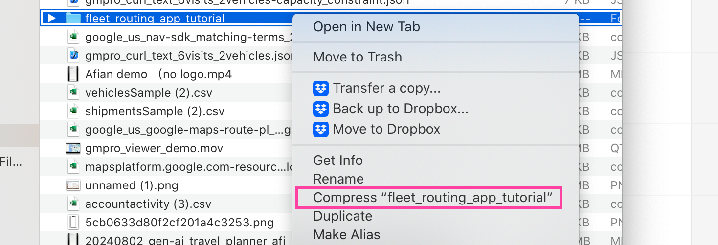
shipments and vehicles sent in the original request to reconstruct the route. Therefore, you need two files: scenario.json and solution.json.Viewing the optimized route plan on the Fleet Routing App
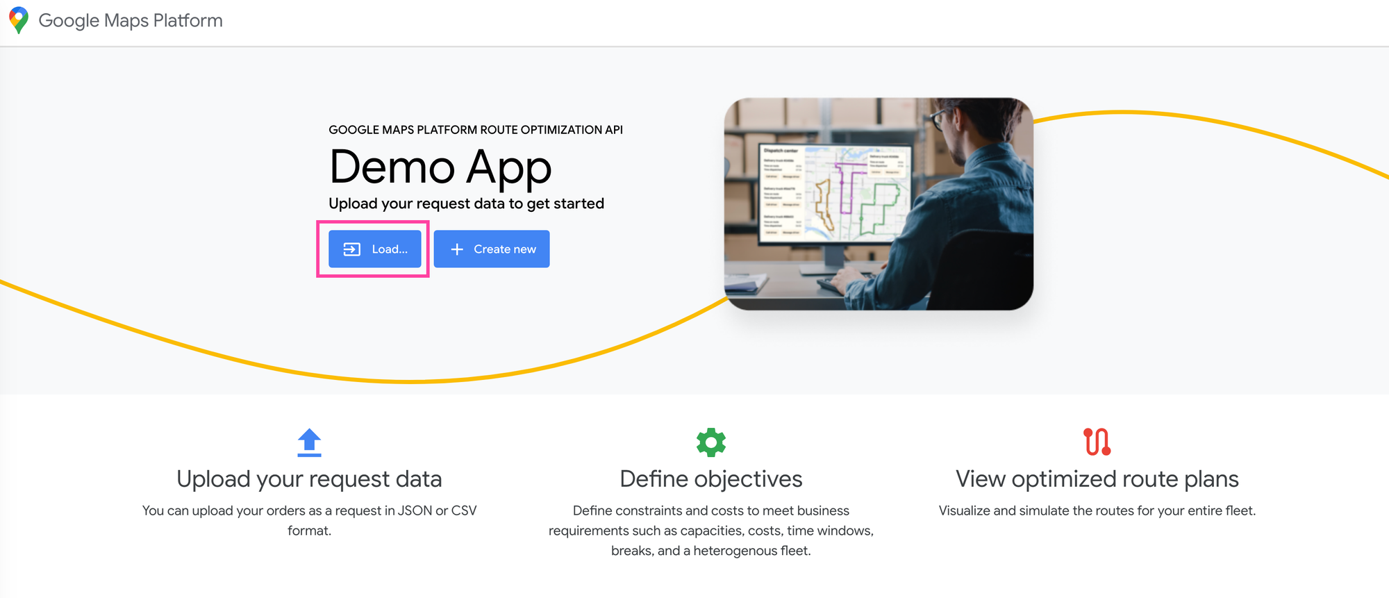
Log in to the Fleet Routing App at https://partners.fleetrouting.app/, and click the [Load] button. If you can't view this page, please contact a Google Maps Partner for access. If you ask nicely, a salesperson will be more than happy to provide you with login credentials.
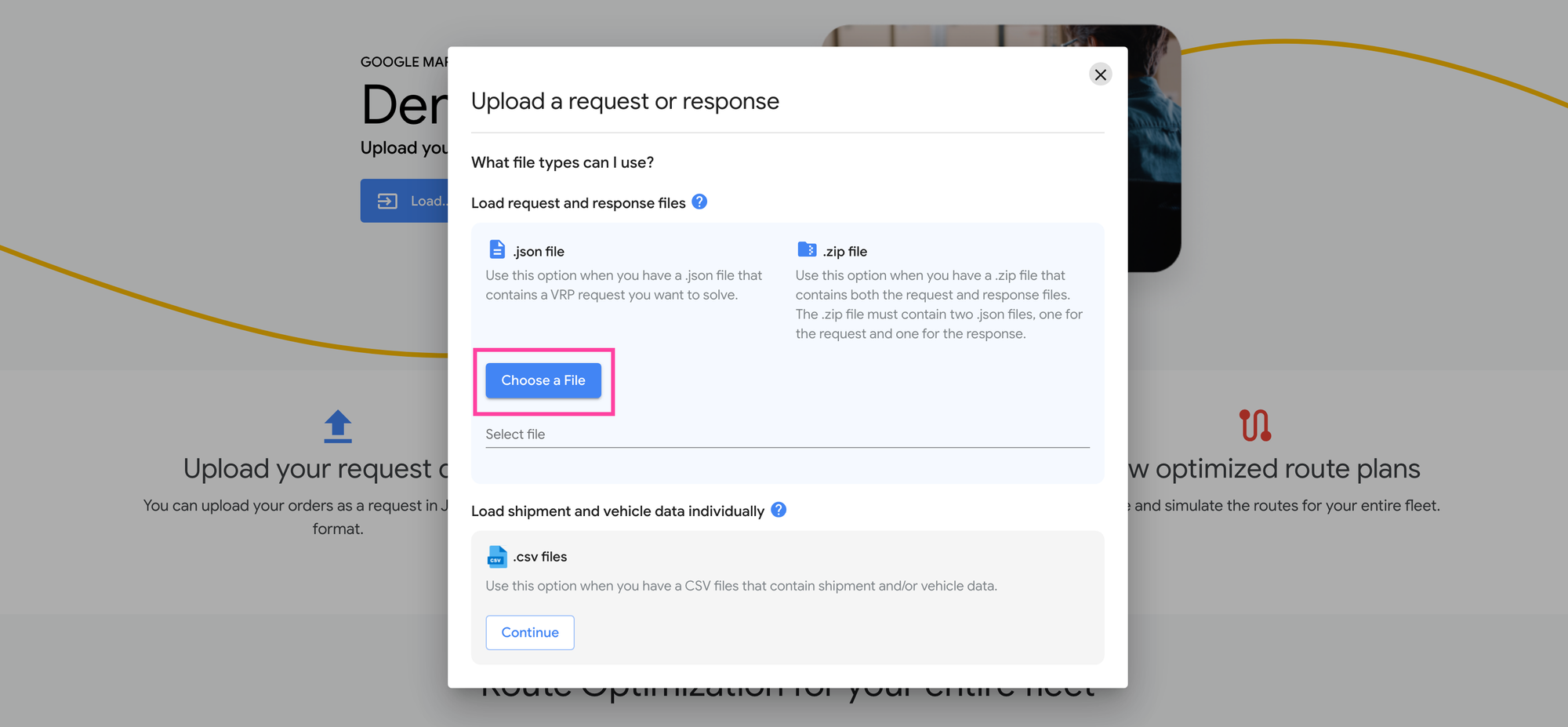
At the popup, click on [Choose a File] and upload the fleet_routing_app_tutorial.zip file you saved to the desktop.
After a few seconds, the optimized route plan will show up.
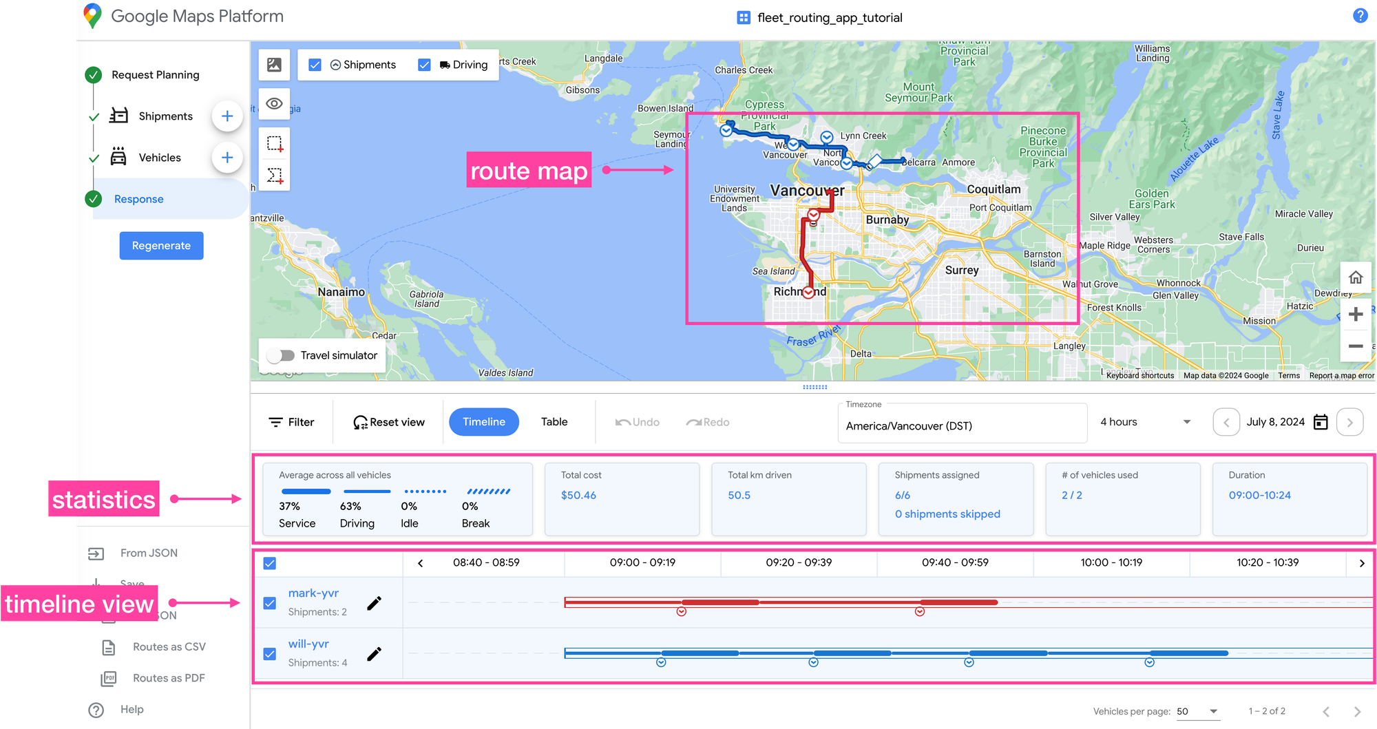
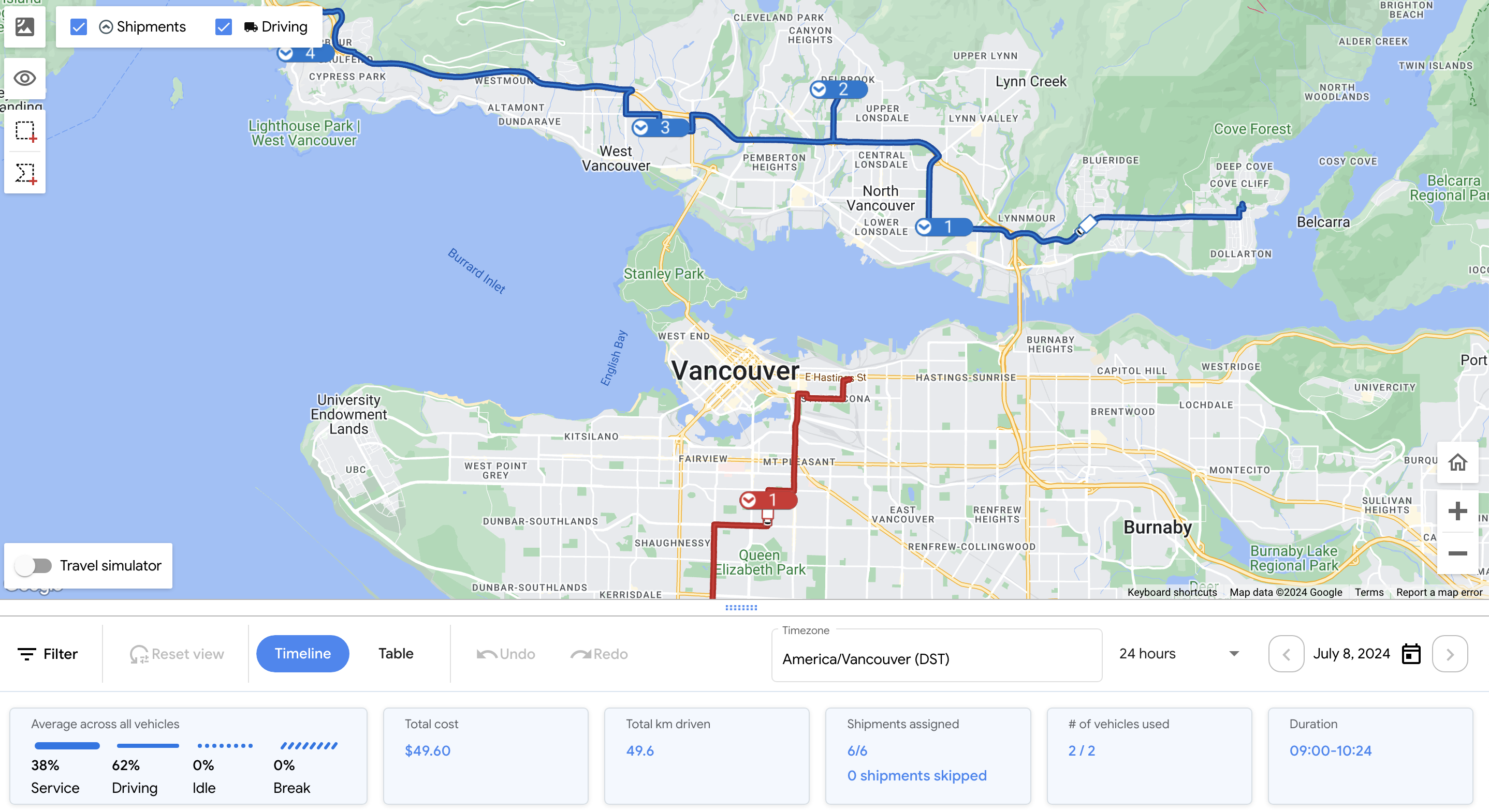
There are three components to the route plan view:
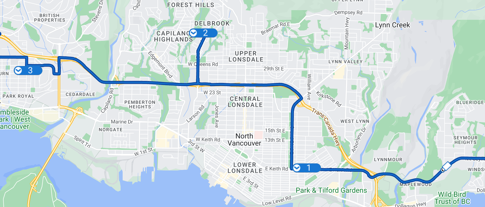
Route map: This displays the optimized routes on an interactive map, with each driver represented by a different color. Deliveries are marked with chevrons (v-shaped symbols), while pickups are marked with carets (^ symbols). The routes for each driver are shown in their respective colors, and the numbers on each marker (visible when you zoom in) indicate the sequence in which the driver should visit each stop.
Statistics: Here you can find aggregate metrics for the route plan, including service time (time spent at each stop), driving time (time spent on the road), and idle time (time spent waiting at a stop for its time window to start). You can also view the total distance driven, the number of shipments assigned or unserved, the number of vehicles used, and the time required to complete all assigned deliveries.
Timeline view: Below the map, a Gantt chart displays the sequence and ETA (Estimated Time of Arrival) for each driver at each stop. A bordered rectangle represents the driver's start and end times, while thin lines indicate time spent driving (transitions), and thick lines represent time spent at a stop (service time).
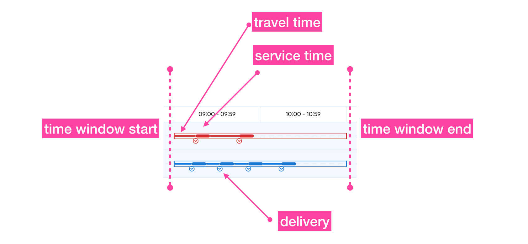
Clicking on each stop in the Gantt chart allows you to step through the route by zooming in on each stop's location one at a time.
Using the Fleet Routing App as a free route planner
In the previous section, we first made an API call to GMPRO and then used the Fleet Routing App to view the optimized routes. In this section, we'll upload shipment and vehicle information to the Fleet Routing App and use it to optimize (using GMPRO in the backend) the routes for us.
Prepare the shipments and vehicles spreadsheets
Instead of using JSON to organize our shipments and vehicles, we'll be using spreadsheets. Each spreadsheet must have the following information:
Shipments
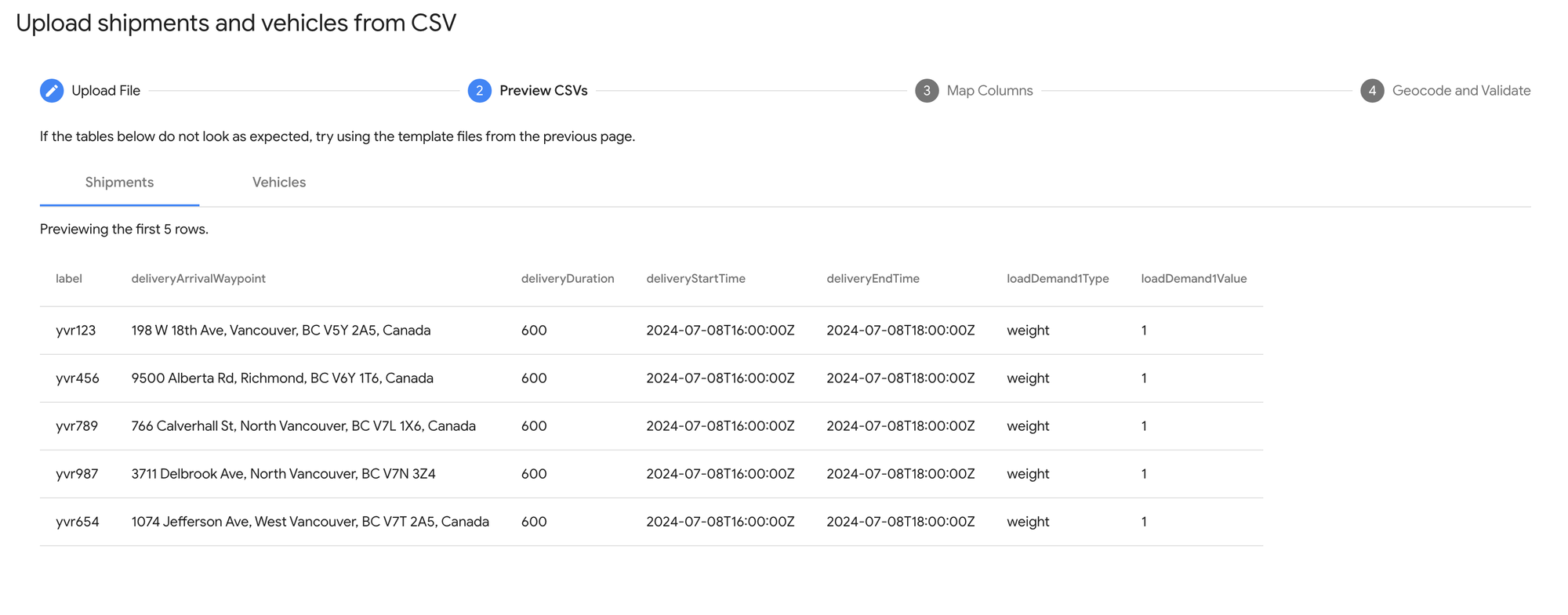
- label: Unique reference number (typically an invoice number) that you use to identify the package.
- deliveryArrivalWaypoint: The address of the customer you are delivering this package to. Make sure to use a full address that includes a zip code e.g. "198 W 18th Ave, Vancouver, BC V5Y 2A5, Canada". Do not put the unit number or any other information in this field.
- deliveryDuration: Also referred to as service time, this is the time (in seconds) spent delivering the package.
- deliveryStartTime: The earliest time in ISO8601 format format that you need to deliver this package. For example, if the delivery address is in Vancouver, Canada (PST) and you need it delivered after 9 am, you should use "2024-07-08T16:00:00Z". 16:00 hrs UTC (Coordinated Universal Time) is 09:00 hrs PST (Pacific Standard Time).
- deliveryEndTime: The latest time in ISO8601 format you need to deliver this package. For example, if the delivery address is in Vancouver, Canada (PST) and you need it delivered before 11 am, you should use "2024-07-08T18:00:00Z". 16:00 hrs UTC (Coordinated Universal Time) is 11:00 hrs PST (Pacific Standard Time).
- loadDemand1Type: The package's unit of load. For example, if the package weighs 1 kg, you would use "weight" for the
loadDemand1Typeand "1" for theloadDemand1Value. Weight and volume are the most common loadDemand types, but you could use any unit of measure you want - "bananas" would work just fine. - loadDemand1Value: The package's load value. For example, if the package weighs 1 kg, you would use "1" for the
loadDemand1Valueand "weight" for theloadDemand1Type.
Vehicles
- label: The name used to identify your vehicle. This could be the driver's name e.g. "Bill" or the license plate of his vehicle e.g. "CA762X".
- travelMode: Either "DRIVING" or "WALKING". Which mode you choose will affect the route taken and the ETAs at each stop (obviously "WALKING" will be much slower than "DRIVING".
- startWaypoint: The start location of the driver. Typically this is the driver's home or the warehouse where packages are consolidated.
- endWaypoint. The end location of the driver. Could be his home or the warehouse, depending on where he parks his vehicle at the end of the day.
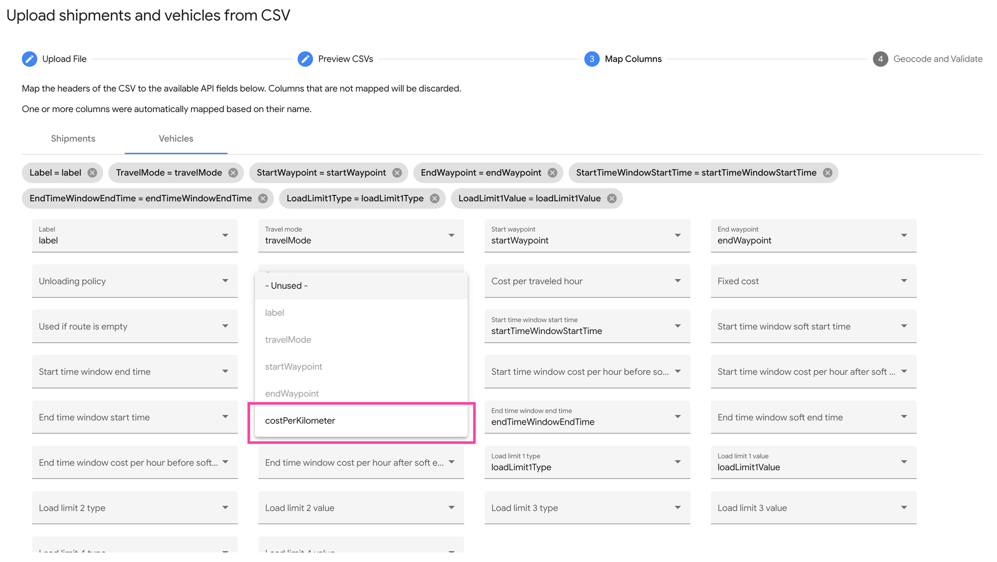
- costPerKilometer: This field sets a baseline for your driving distance costs. GMPRO or any delivery route optimization package is going to try to route as many deliveries as possible for the smallest cost, and if you skip this field the route solution returned will not use the shortest route possible. Note: When we upload the spreadsheet later you'll see that the
costPerKilometerfield is missing, so we'll need to map this to thecostPerHourfield instead. The results shouldn't change much. - startTimeWindowStartTime: The time in ISO8601 format that the driver starts work. This is the earliest time that he can start picking up and delivering packages.
- endTimeWindowEndTime: The time in ISO8601 format that the driver ends work. This is the latest time that he can start picking up and delivering packages.
- loadLimit1Type: The type of load e.g. "weight" constraint used for the vehicle's capacity. Has to match the
loadDemand1Typein the shipments spreadsheet. - loadLimit1Value: The vehicle's capacity value. For instance if your vehicle can carry 5 kg of packages, you would use "5" for the
loadLimit1Valueand "5" forloadLimit1Type.
Upload shipments and vehicles data to the Fleet Routing App
Back at the Fleet Routing App home page, click the [Load] button and choose the "Load shipment and vehicle data individually" option. Click [Continue].
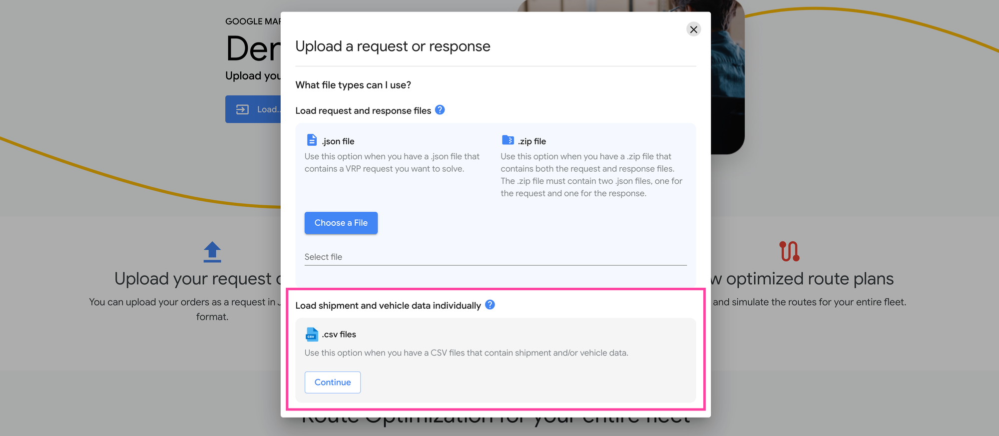
Next, upload the spreadsheet samples provided in the previous section. Both the shipments and vehicles spreadsheets contain the same data as the cURL request used earlier.
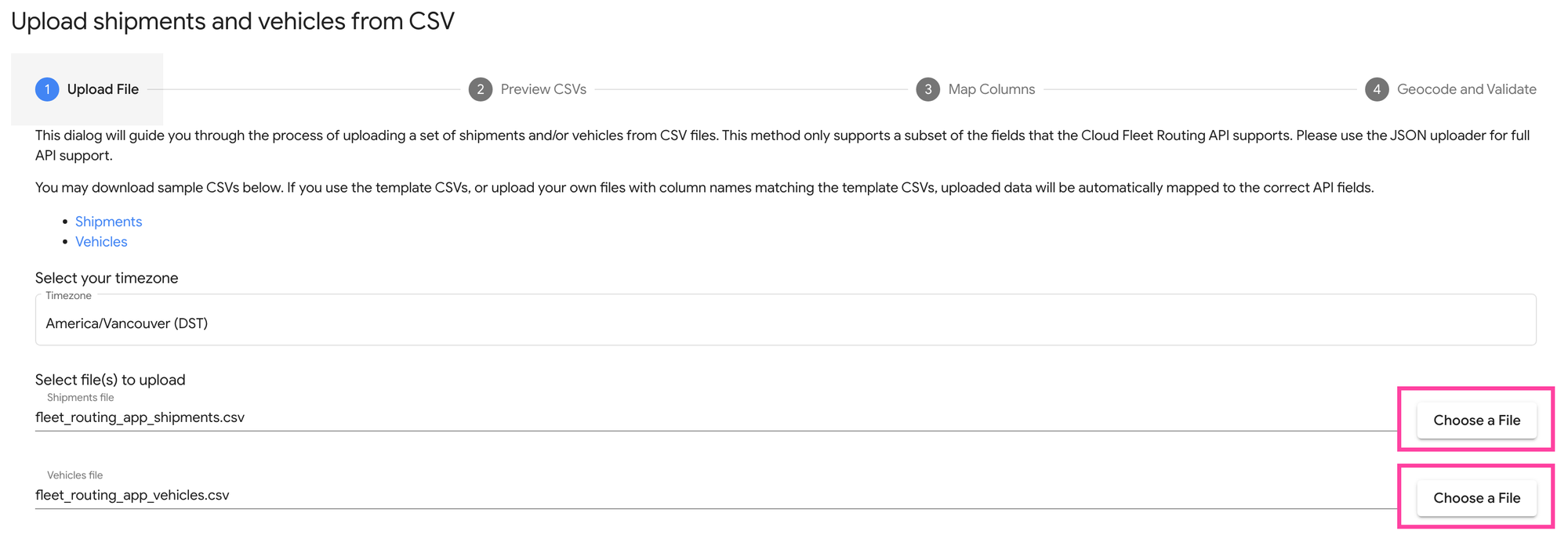
After that's done, review the data to make sure everything got uploaded correctly.
In the next step, we are going to map the columns in our spreadsheets to the fields used by GMPRO. If you used the spreadsheet templates provided in this blog post, this would have been done automatically. The one thing that you must do is map the "Cost per Hour" field to the costPerKilometer column. This way, GMPRO will be able to find the lowest cost solution to the route optimization problem. The "Cost per KM" field in the Fleet Routing App is missing, which is why we have to use this workaround.
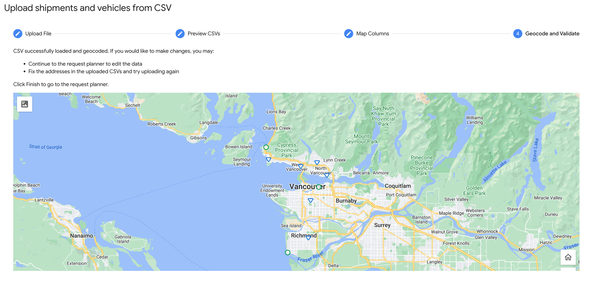
If all this is done correctly, you should get a map with your deliveries displayed as triangles and your driver start and end locations as circle. Select [Finish].
This will return you to the main route planning page. Click [Regenerate] on the left side bar to run the optimization.
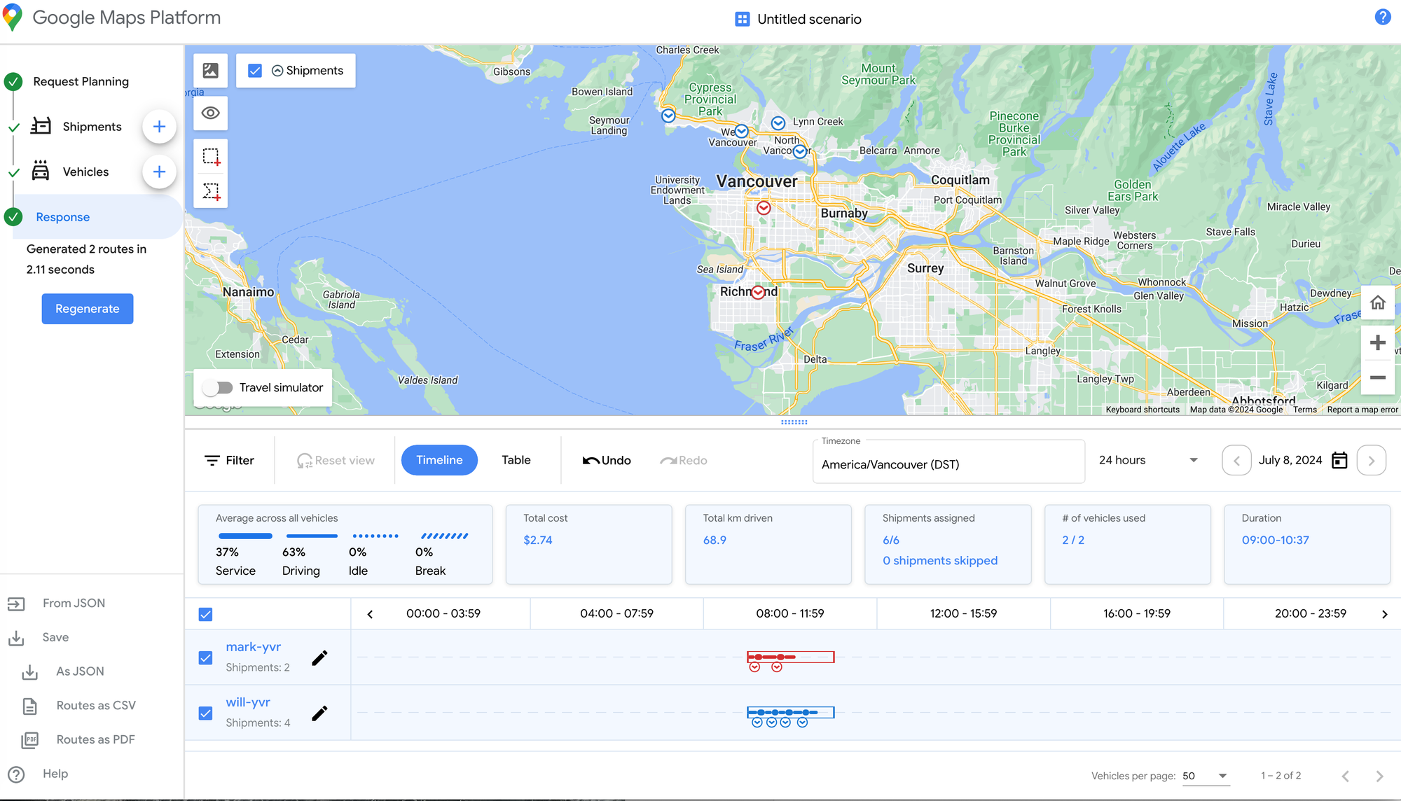
You'll should now be able to see the optimized stops on the map, colored according to the driver that it is assigned to. If you are happy with the results, you can export these GMPRO optimized routes as CSV or PDF files and print them for your drivers. This allows you to use the Fleet Routing App as a free route planner. If you need to tweak something, upload the spreadsheets with slightly different parameters and repeat the process.
Afi Labs can help you build your route optimization system on GMPRO or other Google Maps APIs. 👋 Say Hello! to start working together.
Conclusion and next steps
In this tutorial series on Google's route optimization API, I have demonstrated how to optimize routes using both the API and the Fleet Routing App. We've covered pricing and assessed the pros and cons of incorporating GMPRO as a key part of your route optimization system. In the next few posts, we'll explore how to model your business requirements using GMPRO's advanced features, including pickup and delivery, custom objective functions, soft constraints, cost optimization and territory matching.
👋 As always, if you have any questions or suggestions for me, please reach out or say hello on LinkedIn.

