Google LMFS: Routes Preferred ComputeRouteMatrix API
How to use the Google LMFS: Routes Preferred ComputeRouteMatrix API to return a matrix of distances and travel times.

In this post, I'll run through a worked example of the Routes Preferred ComputeRouteMatrix API and show how you can use it to return a matrix of distances and travel times. Then, I'll use it to solve the assignment problem, a classic problem in combinatorial mathematics involving the optimal matching of agents to tasks in a way that minimizes the total cost of the assignment. The assignment problem can take many forms, but the version that we are interested in here is matching a given number of available taxis (agents) with an equal number of customers (tasks) wishing to be picked up as soon as possible (source code).
Part 1: Google Mobility: An introduction to Google ODRD, LMFS and Cloud Fleet Routing APIs
Part 2: Google ODRD: Routes Preferred ComputeRoutes API
Part 3: Google LMFS: ComputeRouteMatrix API (this article)
Part 4: Google Cloud Fleet Routing: OptimizeTours API
Part 5: Google ODRD: Navigation SDK
LMFS / Routes Preferred ComputeRouteMatrix API example
ComputeRouteMatrix, like its name suggests, is a distance matrix API that computes and returns a "route matrix" - a m x n table of distances and travel times for m origins and n destinations. It improves on Google's original Distance Matrix API by providing faster response times, improved ETA (Estimated Arrival Time) accuracy and incorporating real time traffic. Originally part of Google's Last Mile Fleet Solution (LMFS) route planning and dispatch toolkit, ComputeRouteMatrix is now available as a standalone API when you sign up for Google Mobility.
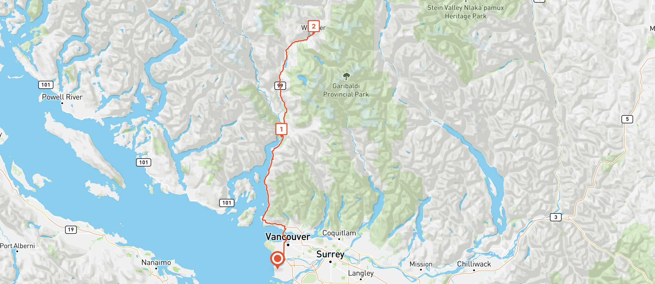
If you visited Vancouver over the summer and wanted to find the travel time from m = 1 Vancouver Airport (49.195,-123.181) to n = 2 Squamish (49.706,-123.150) and Whistler (50.104,-123.084) - both world class destinations for hiking and mountain biking just outside Vancouver, you could make the following call to RoutesPreferred ComputeRouteMatrix API:
Endpoint POST https://routespreferred.googleapis.com/v1alpha:computeRouteMatrix
Headers
Content-Type: application/json
X-Goog-Api-Key: YOUR_API_KEY (contact a Google Maps Partner for access)
X-Goog-FieldMask: originIndex, destinationIndex, duration, distanceMeters
Body
{
    "origins": [
        {
            "waypoint": {
                "location": {
                    "latLng": {
                        "latitude": 49.1951165,
                        "longitude": -123.1814285
                    }
                }
            }
        }
    ],
    "destinations": [
        {
            "waypoint": {
                "location": {
                    "latLng": {
                        "latitude": 49.7069584,
                        "longitude": -123.1507777
                    }
                }
            }
        },
        {
            "waypoint": {
                "location": {
                    "latLng": {
                        "latitude": 50.1042288,
                        "longitude": -123.0840866
                    }
                }
            }
        }
    ],
    "travelMode": "DRIVE",
    "routingPreference": "TRAFFIC_AWARE",
    "departureTime": "2023-10-23T15:00:00Z"
}
origins is an array of origin waypoint objects, each containing the latitude and longitude of the origin location.
destinations is an array of destination waypoint objects, each containing the latitude and longitude of the destination location.
travelMode refers to the mode of transport ("DRIVE", "WALK" or "BICYCLE"). Different modes use different routes (e.g. choosing "BICYCLE" means that the route chosen will prioritize bike paths), have different travel speeds and as such, result in different travel time durations. Note: TRANSIT is not supported in the current version of ComputeRouteMatrix.
routingPreference offers three choices: "TRAFFIC_UNAWARE," "TRAFFIC_AWARE," and "TRAFFIC_AWARE_OPTIMAL." When you select "TRAFFIC_AWARE," the routing algorithm factors in real-time traffic conditions when calculating routes. On the other hand, "TRAFFIC_AWARE_OPTIMAL" also considers traffic but prioritizes speed over absolute precision, resulting in faster route calculations (although slightly less accuracy) due to certain optimizations designed to reduce latency. If you opt for "TRAFFIC_UNAWARE," the routing relies solely on posted speed limits, which means this option is suitable for deliveries in rural areas or cities where traffic congestion is rarely an issue.
departureTime , when combined with routingPreference: "TRAFFIC_AWARE", is probably the single most important field in the input. It allows you to specify the start time of the route as a datetime string in RFC3339 UTC "Zulu" format e.g. "2023-09-25T15:00:00Z" so that the travel time duration returned by the API takes predicted "real time" traffic into account. The "Z" in the string stands for "Zulu" (GMT +0). Since our route is in Vancouver which is on Pacific Standard Time (GMT +7), "2023-10-23T15:00:00Z" resolves to 8 am on Monday, 23rd October, 2023.
Note: If departureTime is left empty, it defaults to the time that the request was made. Also, if you set this value to a time in the past, then the request fails.
The above API call returns the following:
Output
[
    {
        "destinationIndex": 1,
        "distanceMeters": 130439,
        "duration": "7373s"
    },
    {
        "distanceMeters": 78256,
        "duration": "4622s"
    }
]
This looks a bit cryptic, so let's unpack what's going on. A route matrix is essentially a table, with m origin rows and n destinations columns. In this example, there is only m = 1 origins but n = 2 destinations. Because we listed Squamish as the first destination waypoint, it is given a destinationIndex of 0 (which is hidden in the response) while Whistler, being the second waypoint, is given a destinationIndex of 1. Visualized as a table, here's what we get.
| Squamish (0) | Whistler (1) | |
|---|---|---|
| Vancouver Airport | 4622 sec / 78256 m | 7373 sec / 130439 m |
It takes 4622 seconds or 78256 meters to travel from Vancouver Airport to Squamish and 7373 seconds or 130439 meters to travel from Vancouver Apirport to Whistler.
We'd get the same result if we called the RoutesPreferred ComputeRoutes API twice, once for Vancouver Airport - Squamish and again for Vancouver Airport - Whistler. Using ComputeRouteMatrix saved us time because we only need to make a single API call instead of multiple calls to ComputeRoutes.
Solving the assignment problem with the Routes Preferred ComputeRouteMatrix API
Having successfully made a call to the ComputeRouteMatrix API, let's use it to solve the assignment problem.
In the assignment problem, each task must be assigned to exactly one agent, and each agent can handle only one task. The objective is to minimize the total cost or time required for completing all the tasks while ensuring that each task is assigned to a suitable agent. Now that we've formulated the problem, let's see how it applies to taxi dispatch (note: this can also be solved using route optimization, which I've covered in Using route optimization to build a ride share dispatch algorithm).
Problem setup and motivation
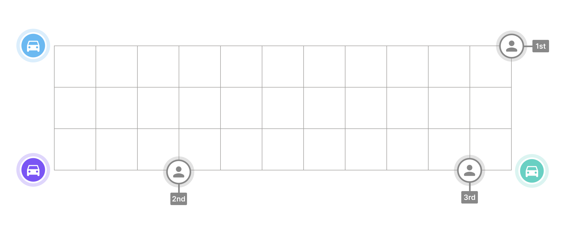
Picture yourself as a dispatcher employed at a taxi company located in Vancouver, Canada. In the midst of a busy workday, you receive three simultaneous booking requests: requests 1, 2 and 3. To figure out which drivers should pick these customers up, you reach for another phone and contact three drivers, blue, purple, and green who are currently available. Plotting both customers and drivers on a grid map of Vancouver (above - each grid is 1 km x 1 km in size), you draw up a distance matrix (below) to enumerate how far each driver is from each passenger.
| Customer 1 | Customer 2 | Customer 3 | |
|---|---|---|---|
| Driver Blue | 11 km | 6 km | 13 km |
| Driver Purple | 14 km | 3 km | 10 km |
| Driver Green | 3 km | 8 km | 1 km |
Because company policy is to ensure that passengers are picked up as quickly as possible, you want to minimize the total time required to pick everyone up.
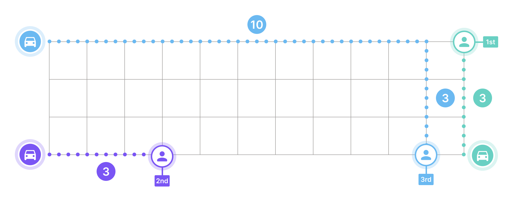
Your first attempt gives a dispatch solution (above) of 1-green, 2-purple and 3-blue with a total distance cost of 3+3+13 = 19 km. Looks OK but maybe there's a better way.
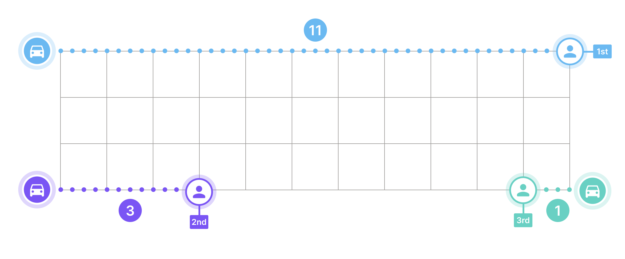
Assigning 1-blue, 2-purple and 3-green (above) gives a much smaller total distance cost of 11+3+1 = 15 km. You keep trying different driver - customer combinations but can't find a better total distance than 15 km - congrats!
Matching agents (drivers) to tasks (customers) is known as the assignment problem, and you solved it using trial and error. It only took you 2 tries to get it right but next time, you might not be as lucky. In general, for a problem with n agents and n tasks. It will take n! tries to find the minimum cost solution. This is because e.g. with 3 drivers and 3 passengers, there are 3 ways to assign customers to the first driver, 2 ways for the next driver and 1 way for the last driver for a total of 3 x 2 x 1 = 6 attempts. For the general case of n drivers and n customers, this adds up to n.(n - 1).(n-2) ... .1 = n!, which is a very big number. For example if n = 8, 8! = 40,320, which will take you the better of the week to solve by hand. Luckily, there are several algorithms such as the Hungarian Method that can solve this problem quickly (understanding how the Hungarian method works is beyond the scope of this tutorial, check out this link if you are interested in the specifics).
In the following sections, we'll use the ComputeRouteMatrix API together with the Hungarian method to solve the assignment problem to optimality.
Generating a distance matrix with the RoutesPreferred ComputeRouteMatrix API
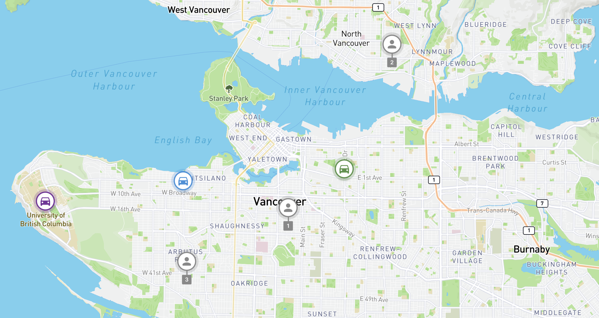
The first step in solving the assignment problem is generating a distance matrix. Instead of a grid map, let's use the city of Vancouver. As in our earlier example, there are three drivers - blue, purple and green that need to be matched to customers 1, 2 and 3 (see map above). Here's what the empty cost matrix looks like:
| C1(49.254,-123.112) | C2(49.313,-123.054) | C3(49.235,-123.169) | |
|---|---|---|---|
| Driver Blue (49.268,-123.183) | - | - | - |
| Driver Purple (49.260,-123.250) | - | - | - |
| Driver Green (49.272,-123.080) | - | - | - |
Let's fill it up by calling RoutesPreferred ComputeRouteMatrix - this time with three origins (drivers) and three destinations (customers):
Endpoint POST https://routespreferred.googleapis.com/v1alpha:computeRouteMatrix
Headers
Content-Type: application/json
X-Goog-Api-Key: YOUR_API_KEY (contact a Google Maps Partner for access)
X-Goog-FieldMask: originIndex, destinationIndex, duration, distanceMeters
Body
{
    "origins": [
        {
            "waypoint": {
                "location": {
                    "latLng": {
                        "latitude": 49.2682989,
                        "longitude": -123.1830924
                    }
                }
            }
        },
        {
            "waypoint": {
                "location": {
                    "latLng": {
                        "latitude": 49.2606086,
                        "longitude": -123.2508593
                    }
                }
            }
        },
        {
            "waypoint": {
                "location": {
                    "latLng": {
                        "latitude": 49.2724384,
                        "longitude": -123.0803332
                    }
                }
            }
        }
    ],
    "destinations": [
        {
            "waypoint": {
                "location": {
                    "latLng": {
                        "latitude": 49.254563,
                        "longitude": -123.1121977
                    }
                }
            }
        },
        {
            "waypoint": {
                "location": {
                    "latLng": {
                        "latitude": 49.3137275,
                        "longitude": -123.0540365
                    }
                }
            }
        },
        {
            "waypoint": {
                "location": {
                    "latLng": {
                        "latitude": 49.2351204,
                        "longitude": -123.1692661
                    }
                }
            }
        }
    ],
    "travelMode": "DRIVE",
    "routingPreference": "TRAFFIC_AWARE",
    "departureTime": "2023-10-23T15:00:00Z"
}
Output
[
    {
        "destinationIndex": 2,
        "status": {},
        "distanceMeters": 5119,
        "duration": "623s"
    },
    {
        "originIndex": 2,
        "destinationIndex": 1,
        "status": {},
        "distanceMeters": 10382,
        "duration": "982s"
    },
    {
        "originIndex": 1,
        "status": {},
        "distanceMeters": 11380,
        "duration": "1150s"
    },
    {
        "status": {},
        "distanceMeters": 7165,
        "duration": "843s"
    },
    {
        "originIndex": 2,
        "status": {},
        "distanceMeters": 4774,
        "duration": "699s"
    },
    {
        "destinationIndex": 1,
        "status": {},
        "distanceMeters": 20051,
        "duration": "1933s"
    },
    {
        "originIndex": 2,
        "destinationIndex": 2,
        "status": {},
        "distanceMeters": 11461,
        "duration": "1363s"
    },
    {
        "originIndex": 1,
        "destinationIndex": 2,
        "status": {},
        "distanceMeters": 7725,
        "duration": "572s"
    },
    {
        "originIndex": 1,
        "destinationIndex": 1,
        "status": {},
        "distanceMeters": 24934,
        "duration": "2288s"
    }
]
Let's parse the output in the form of the cost matrix earlier. Recall that originIndex represents the order in which a waypoint was included in the origins array of the JSON input e.g. Blue (49.2682989,-123.1830924) was the first waypoint, so it has no originIndex value (value is 0), Purple was the second, so it has originIndex: 1 and so on. In the API response, an object with a tuple e.g. {originIndex: 1, destinationIndex: 1} therefore represents the travel time cost of the second origin (Purple) travelling to the the second destination (customer 2). Here's what the returned cost (travel time) matrix looks like:
| C1(49.254,-123.112) | C2(49.313,-123.054) | C3(49.235,-123.169) | |
|---|---|---|---|
| Driver Blue (49.268,-123.183) | 843 sec | 1933 sec | 623 sec |
| Driver Purple (49.260,-123.250) | 1150 sec | 2288 sec | 572 sec |
| Driver Green (49.272,-123.080) | 699 sec | 982 sec | 1363 sec |
In the next section, we are going to use this cost matrix to assign drivers to customers optimally (i.e. minimizing the overall travel time described by the above cost matrix) using the Hungarian method.
Applying the Hungarian method to the ComputeRouteMatrix cost matrix to solve the assignment problem
Instead of manually solving the assignment problem using the Hungarian method, we'll utilize the munkres-js library. This library is named after James Munkres, a Mathematics Professor at MIT who co-invented the Hungarian method along with Harold Kuhn from Princeton University.
First, create a new folder /munkres_solver and in it, create a new file taxi_dispatch_solver.js. In it, add the line:
var munkres = require('munkres-js');
Second, in terminal, cd into your project folder and install munkres-js with this command:
npm install munkres-jsThat's it! You are ready to start using the Hungarian method. Return to taxi_dispatch_solver.js and add the hardcoded travel time matrix costMatrix returned by the ComputeRouteMatrix API (see the previous section) together with pairings, a matrix of text labels for each driver - customer entry e.g. "purple - c2".
const pairings = [
    ["blue - c1", "blue - c2", "blue - c3"],
    ["purple - c1", "purple - c2", "purple - c3"],
    ["green - c1", "green - c2", "green - c3"]
];

const costMatrix = [
    [843, 1933, 623],
    [1150, 2288, 572],
    [699, 982, 1363]
];
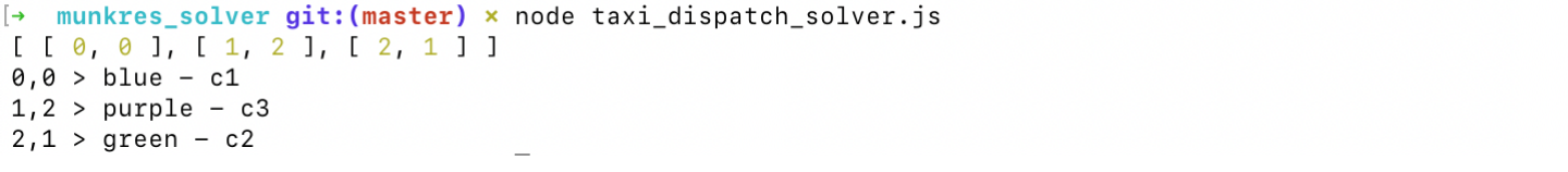
Lastly, run the Hungarian method by calling munkres() and print out the results by running node taxi_dispatch_solver.js on your command line.
const result = munkres(costMatrix);

console.log(result);

for (let i = 0; i < result.length; i++) {
    const driverIdx = result[i][0];
    const customerIdex = result[i][1];
    console.log(result[i] + " > " + pairings[driverIdx][customerIdex]);
}
// => [ [ 0, 0 ], [ 1, 2 ], [ 2, 1 ] ]
If everything went well, you should see the optimal assignment displayed in your terminal window.
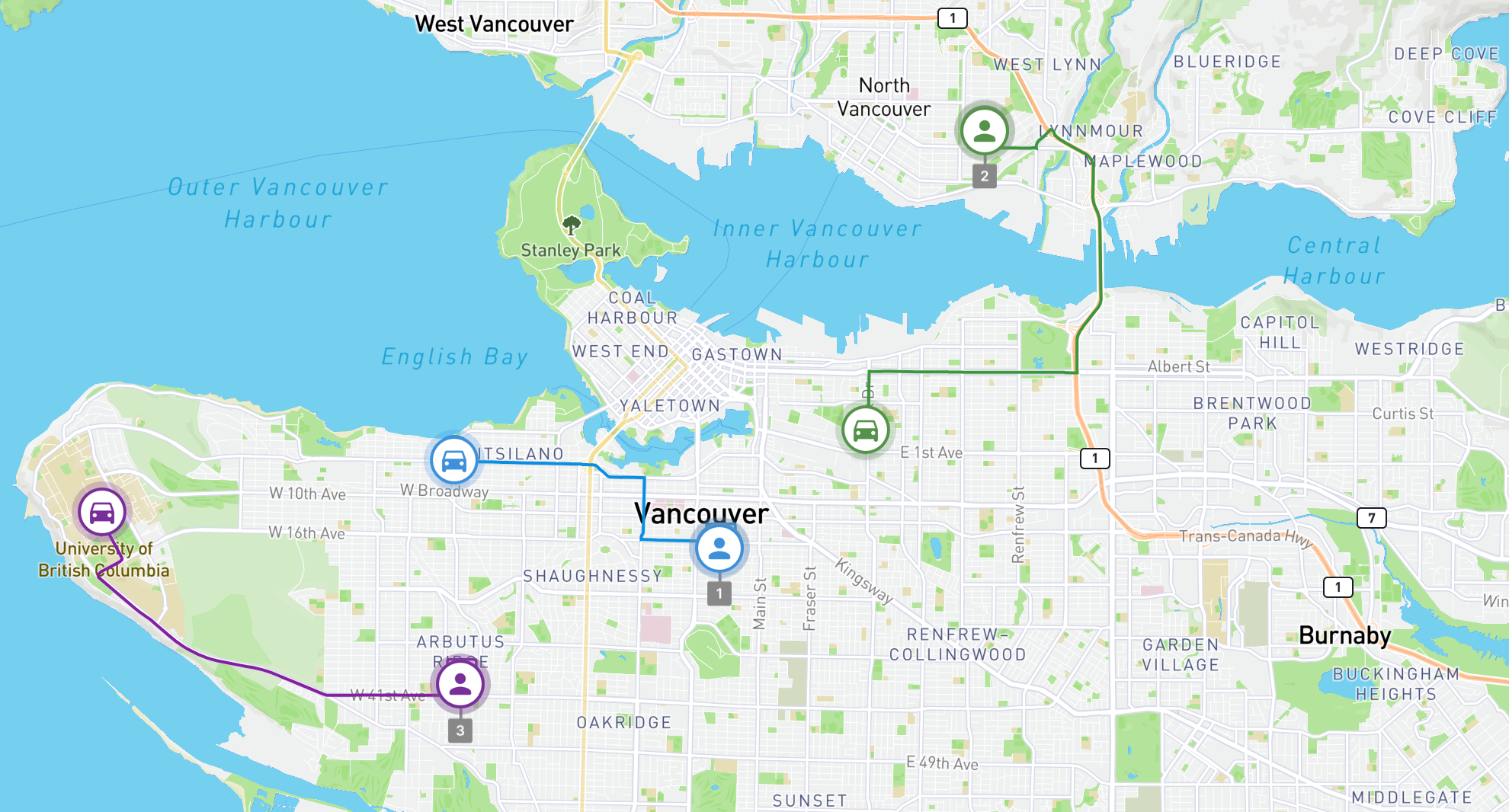
When displayed on a map, the optimal pairings of driver to customer (blue - c1, purpler - c3 and green - c2) make perfect sense. Each driver is assigned to a customer so that the total distance travelled by the overall fleet is minimized.
This concludes my tutorial on the ComputeRouteMatrix API and brief explanation of how you can use it to solve the assignment problem! Similar to other tutorials posted on this blog, the full source code for this project is available on Github.
The ComputeRouteMatrix API is a popular option for logistics companies that already have built their own route optimization engine, but need real time traffic data to improve ETA accuracy and route quality. In the next section, we'll look at how you can combine real time traffic from ComputeRouteMatrix together with best in class route optimization using Cloud Fleet Routing, Google's proprietary route optimization API.
👋 As always, if you have any questions or suggestions for me, please reach out or say hello on LinkedIn.